3. Original use case

3.1. Our data

The data consists of several different scans for 894 patients: CT, PET and MR. The scans have different colour coding. For example, an MR scan will show bone as being dark whereas a CT scan will show bone as being bright which stems from the way the different scans are produced. The scans also have different color codes for air and soft tissue.

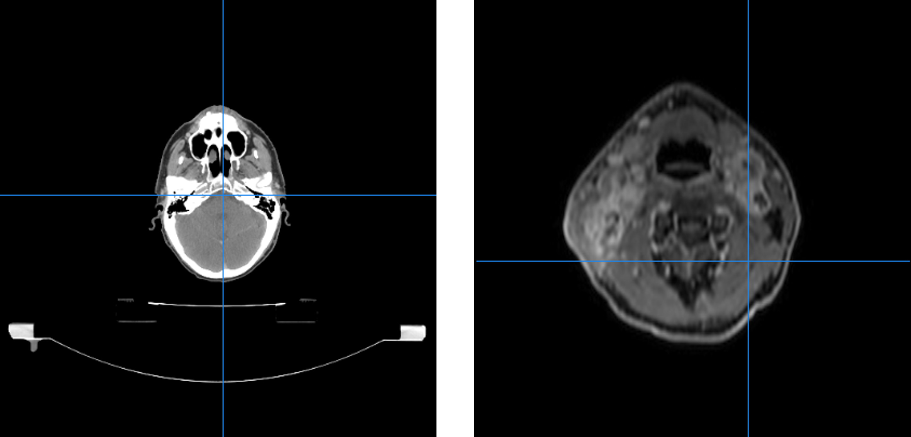
CT- (left) and MR- (right) scan of patient

Thus making it hard to threshold on colour values. Especially on the CT-scans we noise arises in the form of the table the patient is lying on. This can also be seen in the above figure. A potential function would thus have a hard time differentiating between bone and table. Dental fillings can also cause a problem both for CT and MR scans. In CT scans they can cause a sort of flaring whereas in MR they add to the variety of colour codes.

In addition to the images themselves, the data contains various header information, such as the modality of the image, the date of the scan, a medical description of the scan etc. This information is crucial in identifying the scans, referring to them and making decisions about them.

For some of the scans (typically a CT-scan), a doctor has delineated various organs and/or tumours. These delineations are saved as a set of lines in one or more so-called RTSTRUCT-file(s). The RTSTRUCT-file also contains the name of each delineation, e.g. “brain” or “parotid_L” for the left parotid gland. Occasionally, a single organ may have been delineated more than once, e.g. if a patient’s tumour changed in shape or size due to treatment performed between two delineations. In this case, the two delineations will be saved in different RTSTRUCT-files from different dates. The delineations must be kept track of alongside the rest of the data, as they are essentially what an ultimate model must learn from. However, since not all scans have delineations, since not all scans with delinations include the same organs and since not all scans with the same delineations have identical naming schemes for those delineations, identifying the correct delineations is a challenge that must be met.

Our data is thus very heterogeneous as seen with the varying colour coding from scan to scan. Also the different scans are not necessarily positioned equally in proportion to each other. One scan could be located in the top right corner whereas another in the bottom left. The scans also have different dimensions, a feature which impacts cropping. Sometimes a patient doesn’t have both an MR and a CT scan which has to be taken into account when converting. These are all limiting factors when wanting to do comparisons and evaluation.

3.2. Our pipeline and the big picture

The module can be considered as a pipeline which consists of several steps: preprocessing, model development and model usage.

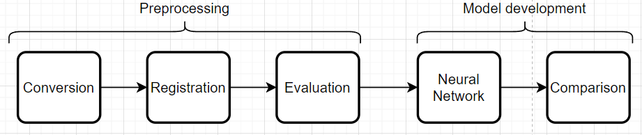
Flowchart of the pipeline

3.2.1. Preprocessing

The preprocessing part of the pipeline handles conversion, registration and evaluation of the registrations. This entails conversion of DICOM-files to the nifti format and afterwards registration of the nifti files. The evaluation is based on a metric score computed from the registrations. In our case, the Mutual Information metric makes sense and having an evaluation threshold at 0.5 is again case specific.

3.2.2. Model development

Model development takes the registered images with an adequate metric score and runs them through a chosen neural network. In our case the neural network nnUNET is used. The idea is then to run the neural network first with CT-scans only and then the registered images consisting of a CT and an MR and then compare. We are dealing with supervised learning since we know what the delineations should look like. nnUNET is an attractive neural network to use since it can figure out the hyperparameters (amount of layers, number of neurons, loss function etc.) given the images and labels.

3.3. Challenges and solutions

This section describes a variety of challenges faced during the project along with the solutions that were developed.

One such challenge concerns the header information in the DICOM-files. When selecting the scans for format conversion, it may at first glance be desirable to select based on the medical description of the scans, e.g. to get an overview of what the scan was used for. However, this is difficult due to the lack of standardisation of those descriptions - in fact, there are occasionally scans which completely lack a description. To overcome this challenge, we have avoided making decisions based on the description, and wrapped the attribute reading in an exception catcher as follows.

        for dicom_attribute in ['Modality', 'PatientID', 'PatientName', 'StudyDate', 'SeriesDescription']:
            if not series_dictionary.get(dicom_attribute, ''):
                try:
                    series_dictionary[dicom_attribute] = str(getattr(dcm_object, dicom_attribute))
                except AttributeError:
                    logger.warning("There exists no attribute " + dicom_attribute + " for file " + str(dicom_filename))
                    series_dictionary[dicom_attribute] = "Default"
                    list_flagged.append((patient_id,"Missing attribute",1))

When writing the dictionary of selected files for conversion to the Excel-sheets, an issue regarding the Excel cell character limit was encountered. For each scan, there is a cell containing the paths to all the files that belong to that scan. However, with some scans having well over hundreds of files, this cell occasionally reached its character limit. To solve this issue, the list of files was instead written to a text file with no character limit, while the filepath to the text file was then recorded in the Excel-sheet cell. This was done for every scan regardless of whether they had enough files to reach the character limit.

A future improvement to this solution would be implementing a database to contain all the filepaths for each scan. This might also be useful to contain the Excel-sheets themselves, however it has not yet been implemented.

The general heterogeneity of the data also poses a challenge, since there are so many edge cases to consider. Some patients do not have a CT-scan with RTSTRUCT-files at all, which consequently means none of the scans for that patient will be selected for conversion. This essentially causes any PET- and MR-scans to be dropped due to a lack of CT-scans with delineations. The opposite is also an issue. If there are several CT-scans with delineations, but no PET- or MR-scans, the selection program cannot be sure which of the CT-scans to choose, since this is usually done by comparing how many PET- or MR-scans relate to the individual CT-scans.

The difficulty of handling edge cases was furthered by the vast size of the dataset, which along with the general complexity of the tasks resulted in very slow code test runs. This issue was with respect to conversion approached by splitting the script into two parts - dictwriter and filewriter, respectively. This eased the testing of potential solutions, since the selection part, which was the most intricate and therefore spanned the most edge cases, was performed in dictwriter while the heavy file format conversion itself was performed in filewriter. Essentially, edge case solutions could now be tested without immediately committing to performing the computationally expensive part of this task.

A similarly resource-diminishing approach would be very desirable for the registration task, which requires even more compute. However, in this task, it is more difficult to evaluate solutions without simply running the entirety of the script, i.e. the only feasible route by which to see the effects of a given solution is to implement it and consider the results afterwards.

In proportion to evaluation of registered images thresholding on a color value was considered but noise in the form of tables and dental fillings proved this procedure to be more complicated than first anticipated. We wished to evaluate using a dice coefficient. Thus it was necessary to produce a mask so unwanted pixels didn’t come into play when evaluating. The idea was to let all pixels with a value larger than zero, where a value of zero equals air, constitute the mask. A table would have a value larger than zero but it would not be desirable to include in the evaluation. Also the dice coefficient is vulnerable to varying volumes of the scanned object. These two issues caused us to use another evaluation method and metric.

The solution was instead a mix of thresholding on color value and croppping the images using a cropbox. The cropbox minimizes the amount of pixels with a value of zero by cropping as close as possible around the desired region. Thus it will never crop away values that are larger than zero which we want to keep. This means pixels that constitute air are still a part of the evaluation but the problem has been minimized. We always crop based on the MR image meaning noise such as a table is not included in the cropped image. This is because the table does not show up on an MR-scan and the MR-scans have smaller dimensions than the CT-scans meaning it would be cropped no matter what. The metric used for evaluation was changed to Mutual Information instead since producing a mask that only includes values larger than zero was impractical.

Again in proportion to evaluation an idea was to look at differences in the color value sum for each slice in an MR-scan. Thus we would calculate the value sum of a slice and then take the next slice and calculate the sum again. If the difference in the two sums were large enough, that is above a certain threshold we crop the image at that slice since a large difference in sums would mean going from air to tissue. The problem was finding a threshold applicable to all patients. This proved impossible since the starting slice is not always located the same place for each scan meaning if the starting slice is the side of the patients head we would never achieve a high difference in sums.